Material and model setup

When a project is initialised it is then possible to define material and set the model.

Let us first look at the general layout of the Model page, which is split up into two parts, the main window showing the graphs and the sidebar being the control panel for variables and data.

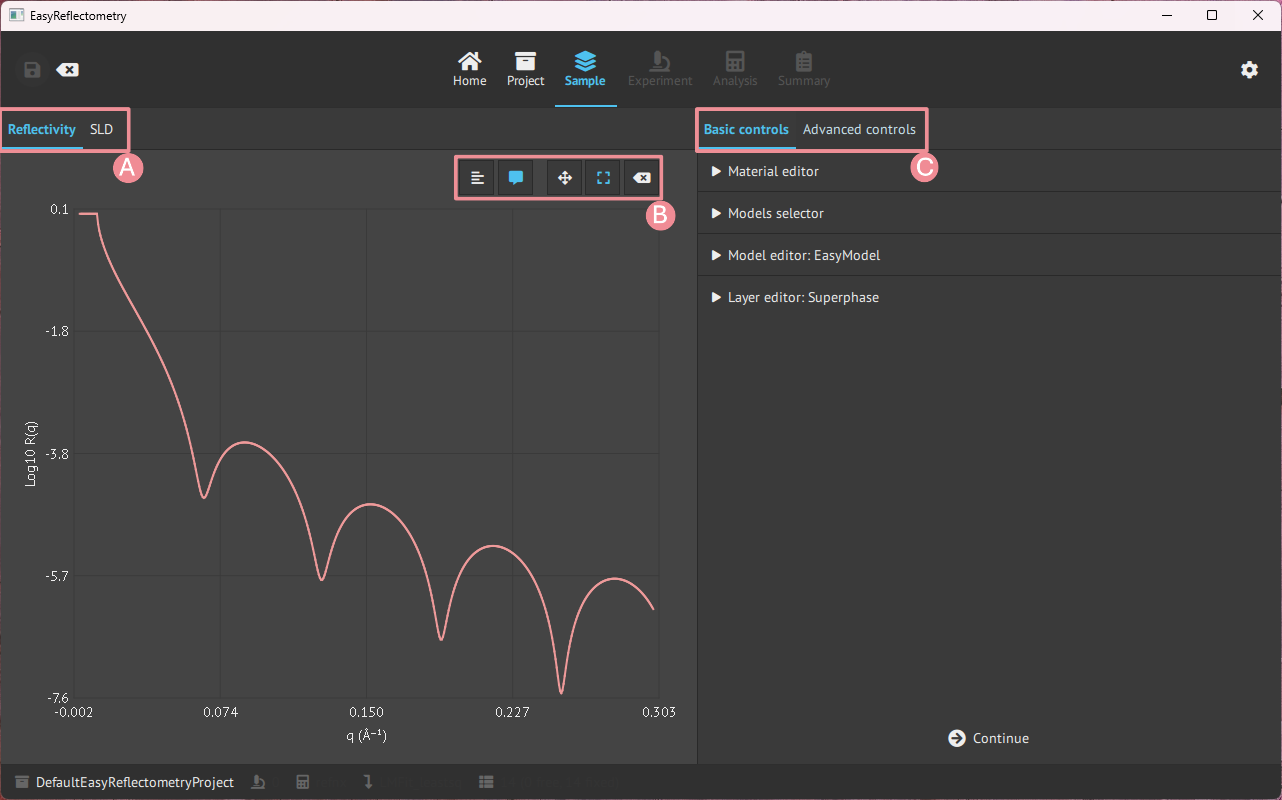
• A: Graph change between the Reflectivity- and Scattering Length Density (SLD) curve.

• B: Graph control of ledger, visible coordinates on hower, zoom and pan control, and reset.

• C: Basic controls, for defining material and model, and advanced controls for further setting parameters.

Basic controls

Material editor

To construct a model in the app, first, you add the materials that will compose the layers in Material Editor.
The materials are added by the real and imaginary components of the scattering length density (in units of 10^-6Å^-2) and given a name for the material.

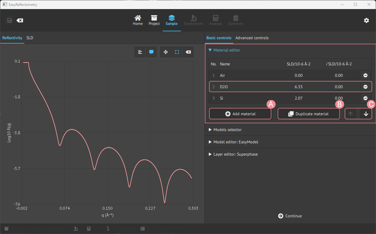
• A: For adding more material.

• B: Duplicating the last clicked material.

• C: Changes the ordering of materials.

Model creation and editing

For creating new models, the Models selector tab is used, and then for setting the assemblies in the model the Model editor is used.

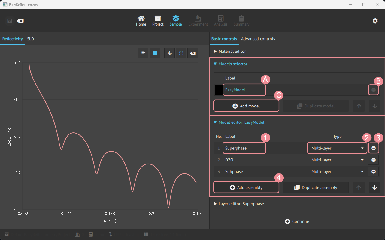
• A: Renaming model.

• B: Removing the specific model.

• C: Adding more models.

• 1: Renaming/naming the assembly.

• 2: Setting the type of assembly; Multilayer, Repeating Multilayer or Surfactant layer.

• 3: Removing the specific assembly.

• 4: Adding more asseblies.

Layer editor

Then for editing the assemblies in the model, the Layer editor is used.
By clicking an assembly, the Layer editor is specified and changes can be made to that assembly.

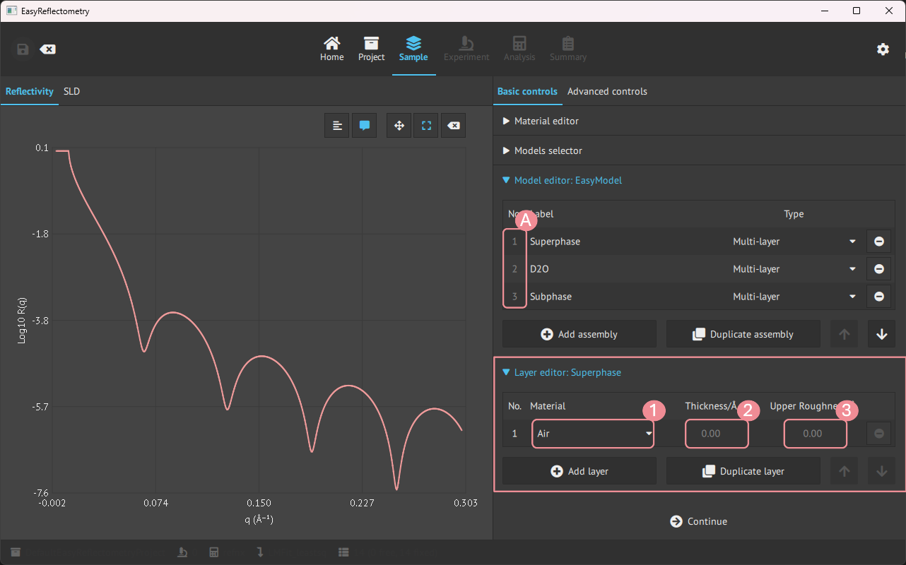
• A: Pick the desired assembly to modify.

• 1: Choose a material from materials in the Material Editor.

• 2+3: Setting the Thickness and Upper Roughness of the material in Angstrom, Å.

Magnetism

A layer can also be given a magnetisation, in the Magnetism group below the layer editor. This needs the refl1d calculation engine and is described in magnetic layers.

Structure view

The main window has a Structure tab next to Reflectivity showing a schematic of the current model’s layer stack: one colored box per layer, ambient medium on top, substrate at the bottom. Boxes share a color per material (see the legend), box heights follow layer thickness, and repeated multilayers with many repetitions are drawn once with a “× N” badge.

Hover a box for its material, SLD, thickness and roughness; click it to select that layer in the sidebar editor. The view updates immediately when the model changes, including after a fit.

Note the view is a schematic, not a to-scale cross-section: heights are clamped so very thin layers stay visible and very thick ones do not crowd out the rest.

Advanced controls

In the advanced controls, it is possible to apply a specific Q-range of interest, to choose the calculation engine, and to constrain the parameters of the model.

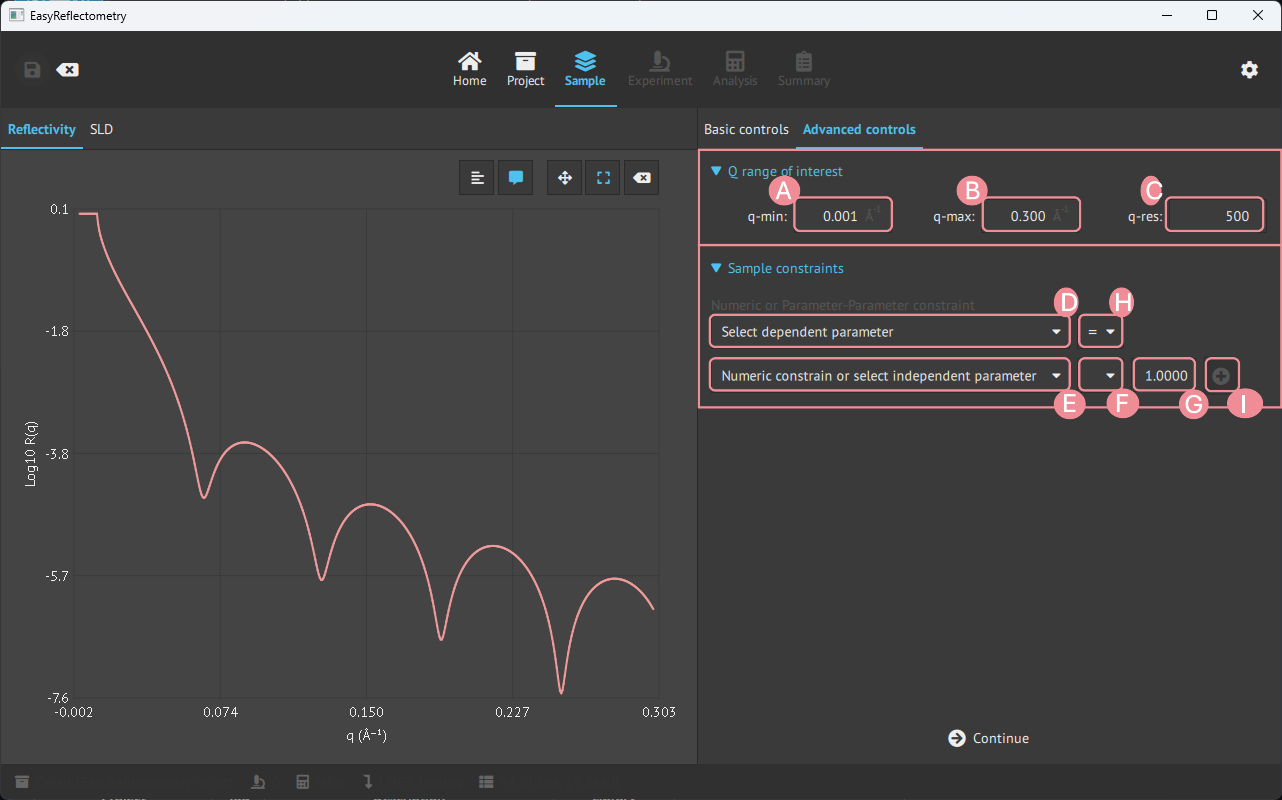
• A: Setting min. Q value of interest.

• B: Setting max. Q value of interest.

• C: Setting Q-resolution.

The Calculation engine group selects between refnx and refl1d for this project. The same selector is available on the Analysis page. Only refl1d can model magnetic layers, so selecting refnx while the sample has magnetic layers is refused - see magnetic layers.

Below these sit three constraint groups, from the most specific to the most general.

Physics constraints

The Physics constraints group applies physically motivated constraints to an assembly with one click. The list is per assembly of the current model, and only shows the recipes that make sense for that assembly type; a recipe that cannot be applied right now is marked n/a with the reason, and one that is always in force is marked always on.

Recipe	Effect
Conformal roughness	Every interface of the assembly shares the roughness of its first layer.
Conformal thickness	Every layer of the assembly shares the thickness of its first layer.
Constant period Λ	The summed thickness of the layers stays constant: the last layer absorbs whatever the others change by.
Equal head/tail area per molecule	The head layer takes the area per molecule of the tail layer (surfactant layers).
Symmetric head groups	The back head layer follows the front head layer thickness and area per molecule (bilayers).
Solvent roughness follows the surfactant	The roughness of the first layer below the surfactant follows the tail roughness. Needs Conformal roughness.
Mixture fractions sum to 1	Material mixtures and solvated materials keep their fractions normalised. Always on, not toggleable.

Each active recipe appears as a single row in the Active Constraints table of the Single constraints group, of type physics, counting the parameters it ties together.

Single constraints

The Single constraints group creates numeric or symbolic relationships between individual parameters.

1. Pick the dependent parameter from the drop-down.

2. Pick the relation: =, ≤ or ≥.

3. Type the expression, for example np.sqrt(1 / sld_ni) + 4. Use Insert parameter alias… to paste the alias of another parameter rather than typing it, and Insert total film thickness to use the read-only sum of all layer thicknesses between superphase and subphase.

4. Check the Preview line, which shows how the constraint will read - and, for an inequality, that numeric literals are interpreted in the dependent parameter’s unit.

5. Press Add constraint.

= ties the parameter to the expression, so it is no longer free. ≤ and ≥ against other parameters become inequality constraints, which are enforced as penalties during fitting.

Warning

Inequality constraints need a BUMPS minimizer (Analysis › Minimization method). With lmfit or DFO-LS selected the group shows a warning and fits are refused until the minimizer is changed or the inequality is removed. A warning also appears when the current parameter values violate an inequality, and again fits will not start until they hold.

Existing constraints are listed in the Active Constraints table, with columns No., Type, Parameter and Expression. The Type column tells the kinds apart - expr for a plain equality, ≤ ≥ for an inequality, physics for a recipe from the group above, bound for an upper bound and value for a fixed value - and each row can be removed individually.

Model constraints

The Model constraints group ties whole models together rather than single parameters: select two or more models and press Constrain models parameters to constrain all of their matching parameters at once. This is the tool for co-refining several contrasts that share a structure. The resulting constraints are listed in the Model Constraints table below the selector and can be removed there.

Trying the constraints out

Four simulated datasets with a known ground truth are provided for exercising these features - see demo datasets.