Simple fitting with a slab model

For this purpose, we have created a simple slab model which is discussed in detail in the model-dependent analysis and reflectometry slab models sections of the ISIS Virtual Reflectometry Training Course on neutron reflectometry fitting.

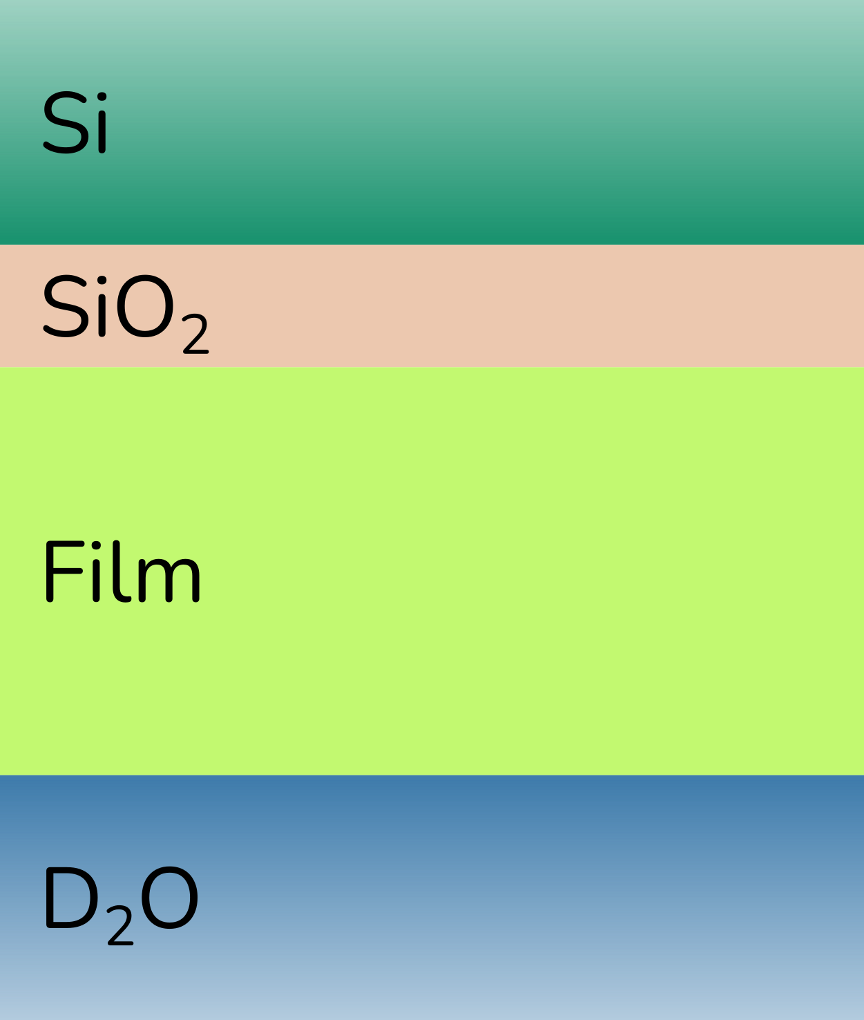
The system that we are investigating consists of four layers (with the top and bottom as semi-finite super- and sub-phases). The super-phase (where the neutrons are incident first) is a silicon (Si) wafer and as a process of the sample preparation, there is anticipated to be a layer of silicon dioxide (SiO₂) on this material. Then a polymer film is attached to the silicon dioxide by some chemical method and this polymer film is solvated in heavy water (D₂O) which also makes up the sub-phase of the system. This is shown pictorially below, as a slab model.

Now for explaining the Analysis tab let’s look at how the EasyReflectometryApp can fit. The tab is like the previous tabs split into two windows, a graph- and a data-window.
The graph window has the same functionality as the previous tabs, so it will not be explained further. The data window has two categories: Basic and Advanced controls.

Basic controls

The basic controls is for fitting the variables.

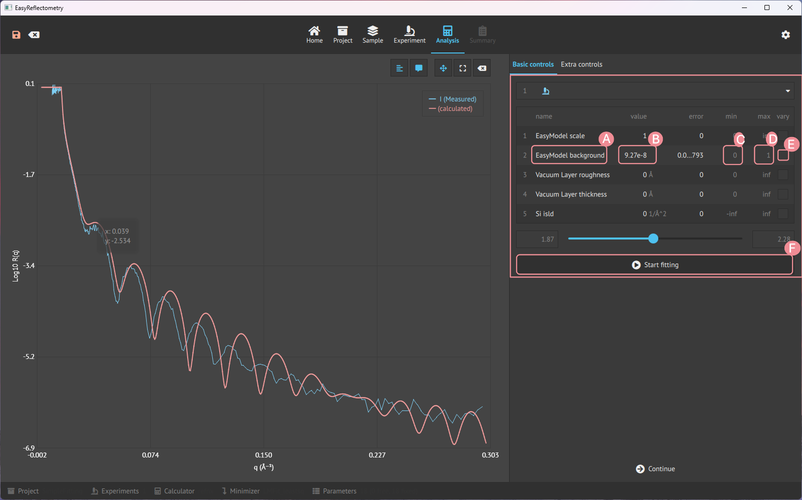
• A: Picking the desired variable to use the slider for fine-tuning it.

• B: Able to change the specific variable.

• C: Setting the minimum variable for fitting.

• D: Setting the maximum variable for fitting.

• E: Choose the variable for fitting.

• F: Fit the chosen variable (E) between the min. (C) and max. (D).

Advanced controls

The advanced control is then for changing the calculation engine and setting the minimisation method.

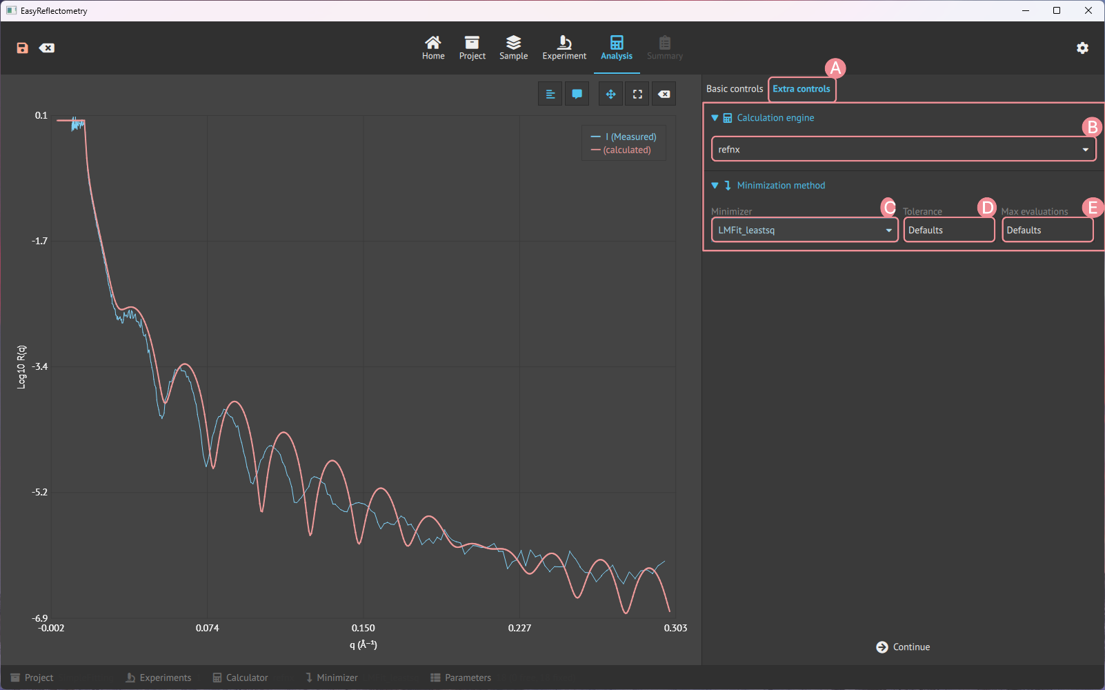
• A: Changing the calculation engine between refnx and refl1d.
  
  

• B: Setting the minimisation method for minimising variables.

• C: Specifying the tolerance of the set minimiser.

• D: Setting the maximum number of iterations(evaluations) for the minimiser to run.

The calculation engine (A) is also available on the Model page, in its advanced controls; both selectors change the same project setting. Note that only refl1d can model magnetic layers, so a sample with magnetism cannot be calculated with refnx - see magnetic layers.

The first entry of the minimiser list (B), BUMPS-DREAM (Bayesian), does not minimise but samples the posterior distribution of the fitted parameters; it replaces C and D with its own sampling settings. See Bayesian analysis.

Residuals

The lower panel of the Analysis page has three tabs: SLD, Residuals and, for a polarised experiment that measured both non-spin-flip channels, Spin asymmetry.

The Residuals tab plots the weighted residual (M-E)/σ against q - the difference between the model and the experiment, in units of the measured uncertainty. A good fit scatters evenly around zero with no structure left in it; a systematic wave or a drift means the model is missing something. The tab has the same legend, hover, zoom, pan and reset controls as the other charts, and its q-axis follows the logarithmic setting of the reflectivity chart.

With several experiments, or with a polarised experiment, the tab draws one residual curve per visible measured series. A spin channel the model cannot calculate contributes no residuals.